Nanopore RNA Sequencing Protocol
! WARNING
This protocol is explicitly for the new SQK-RNA004 Nanopore kit. If you are using the discontinued SQK-RNA002 kit and either an R9.4.1 flow cell or flongle, please see the old Nanopore RNA Sequencing Protocol (SQK-RNA002).
This pipeline is the basis for Nanoswift (Version < 0.1.0 alpha), an application that will automatically perform all of the work and analyses you see here (except, of course, for the wet lab portion) and upload the results. If you have access to Nanoswift (Version > 0.2.0 alpha), you may use it instead of the Sequencing (which includes alignment and formatting) and m6A Detection sections below.
Also, this protocol is written with the intention that you are on a Linux-based machine, Ubuntu in particular. Certain things may be different for you, such as installing dependencies, if you are not on a Ubuntu machine. If you are trying to run the pipeline from Windows, I recommend that you use the Windows Subsystem for Linux (WSL). MacOS users should be able to follow along very closely, as I will use Conda for a lot of the command-line application installs, but some dependencies will need to be installed through Homebrew and some file paths may be different. Keep in mind that most of these command-line applications are written for the x86 architecture, and so if you are on a Mac with an Apple Silicon ARM processor, you will need to run Terminal through Rosetta 2. This can be achieved by right-clicking Terminal, selecting Get Info, and ticking the Open using Rosetta option, and can be checked with the uname -m command in the shell. Some applications may have an Apple Silicon ARM processor version.
For m6A Detection, this guide currently uses m6ANet, however, Dorado now supports native m6A detection. I plan to integrate Dorado m6A detection into this protocol at a later date for comparison. Like its predecessor Guppy, Dorado can utilize CUDA enabled GPUs for faster basecalling. You may want to cross reference your GPU with the list of CUDA compute capabilities here.
Introduction
Hello, and welcome to the mRNA m6A modification detection guide and protocol. This protocol is a fully comprehensive guide designed to help you get a Linux (or compatible shell) computer up and running from scratch for m6A mRNA modification detection using direct Nanopore sequencing. The initial goal of this project was to detect m6A mRNA modifications in glioma samples, the coveted glioma mRNA m6A Methylator Phenotype (or “G-RAMP”), analogous to epigenetic modifications at CpG sites in glioma (glioma CpG Island Methylator Phenotype, or “G-CIMP”). However, this protocol can be used to detect any m6A mRNA modifications in a sample, with a few minor modifications. With all of this in mind, I have written this protocol in as a generic way as possible, describing everything I can along the way, so that hopefully anyone reading this can replicate what I’ve done without any R knowledge or computer programming experience. Some of the code may be intimidating at times, but I will try to explain each syntax as I go along so that you can understand what each line is doing as you move through the code.
This protocol is separated into six major sections: Introduction, Requirements (and Installations, if necessary), Running Samples (wet lab portion), Sequencing, m6A Detection, and Final Analysis. Each of these sections utilize different skills and/or software for processing samples and data (for example, sequencing and alignment will be handled via Dorado and minimap2, while m6A detection will be handled via m6ANet), which will be outlined at the start of the protocol. Where applicable, I will include warning boxes to help you avoid running into errors, and should never be glossed over when doing a run. Other bits of information that are not as paramount to a successful run will be included in block quotes. At the end of the protocol, I will also include an Appendix section, which will contain technical terms that will be used throughout the guide and an Additional Information section containing useful information about the nanopore system itself.
Finally, a big shoutout to Bryan Kevan and Sean Pianka, who laid down the ground work for this project, Albert Lai for his support and encouragement, Luca Cozzuto and the Goeke lab for their help in troubleshooting at challenging steps of getting the pipeline up to speed, and the latter for the development of m6ANet. Without them, this project would not have been possible.
Without further adieu, let’s get to it!
Defining Files
In an effort to make this pipeline as generally applicable as possible, I thought it best to start by defining where everything is on your computer first so that you can just call these shorthands in the Terminal later. This will also allow you to simply copy and paste the code from the code blocks below, without having to change anything in the code itself for it to work. The locations we will need to define are as follows:
- The location of your Dorado installation and the bin folder at
root/dorado-0.6.2/bin. We will call in Terminal with$DORADO. Note that your Dorado version may be different from mine, and thus you will need to change the0.6.2to whatever it is. - The location of where you want to store the Dorado output as a log text file, if desired (in case you need to refer to it at some later point). We will call this with
$DLOGS. - The location of where you will store your reference transcriptome (or genome) files. This will be called with
$REF. - The locations of your raw nanopore
.fast5data, where you want to store the basecalled.fastqdata, and where you want to store the aligned.sam,.bam, f5c/Nanopolish output data. We will define these as$NRAW,$NBASE, and$NALI, respectively.
Note
Dorado is faster with .pod5 files as input, but that may be incompatible with f5c/Nanopolish and m6ANet down the pipeline. For this reason, I keep the raw files in .fast5 format, even though it is suboptimal. Additionally, .pod5 is now the default file format exported from the MinKNOW software. You may want to change that during the sequencing run, or convert it using ONT's pod5 software.
- The location of the m6ANet folder where you want to store the working and output files. We will call this with
$M6AO.
Note that for my installation, I will put all of these in a folder labeled /Research within my /home/ directory. If you do the same, you can call this base directory with the string /home/$USER/Research (Linux only; it depends on your operating system), regardless of what your unique username actually is. In addition, at the start of each run, I will define the name of my sample (currently by flow cell ID), which will be the same name as the folder that contains my raw .fast5 reads in my Nanopore raw data folder. This string (SAMPLEID) will be used to fill in file names and folder names as we go along, so you shouldn’t have to edit any of the code as you do more samples. We will do the same for the reference transcriptome file.
! WARNING
If you do additional runs and re-run this pipeline, you will need to change the SAMPLEID and execute the following code block each time before running the pipeline. Otherwise, you will overwrite the data from your last run! Additionally, you will need to redefine these variables each time you open a new Terminal window. If you do not have any of these software installed yet, I recommend coming back to this section and running this code after you have the appropriate software installed.
Shell File Paths
Tip
You can easily find out what your current working directory is in the Terminal by typing echo $PWD and hitting execute. Similarly, you can define your current directory as a variable by setting your variable equal to $PWD. PWD stands for print working directory and is a shortcut that will benefit you a lot as you navigate and define folder directories in the shell.
Bash
SAMPLEID="FAR91556" \
GREFERENCEID="GRCh38.p14.rna.fna" \
DORADOVER="0.6.2" \
DORADO="/home/$USER/Research/dorado-${DORADOVER}/bin" \
DLOGS="/home/$USER/Research/logs/dorado" \
REF="/home/$USER/Research/Ref" \
NRAW="/home/$USER/Research/Data/Nanopore/Raw" \
NBASE="/home/$USER/Research/Data/Nanopore/Basecalled" \
NALI="/home/$USER/Research/Data/Nanopore/Aligned" \
M6AO="/home/$USER/Research/Data/Nanopore/m6ANet_results"
Know that at any time, you can check these in Terminal using the echo command. For example, if I wanted to check what my current SAMPLEID was, I would type echo "${SAMPLEID}" and execute.
Requirements
Note
If you already have a system up and running with the necessary software and hardware, you may skip ahead to the Running Samples or Sequencing sections for processing data.
In order to acquire Nanopore data and properly analyze it, we need to ensure that our pipeline has all the necessary hardware and software packages installed on our computer before we can begin analyzing samples with the pipeline. Here is a list of things you will need to proceed further:
Hardware
- A computer with a strong CPU/GPU running a Unix-based system (either Linux Ubuntu 18+, macOS 10.11+ El Capitan, or WSL). For this guide, we will assume you are running Linux with a CUDA enabled GPU, but you should be able to follow along on Mac as well (just know that some of the paths may be different to your files, you may need to download slightly different packages, and your system may process files slower). You can also use Windows via WSL, but I will not be covering how to set that up in this guide. If you wish to do that, install WSL on Windows as described here first and then follow the guide as if you were on a Linux machine.
- 30 GB minimum of RAM (although ideally 64+, since 30 GB will be needed on top of the available RAM for the OS to basecall with Dorado). You can go lower in RAM, but I generally don’t recommend it.
- A MinION Mk1B Nanopore.
- An RNA flow cell.
- A SQK-RNA004 Direct RNA Sequencing Kit.
Additional reagents may be required for the wet lab portion for RNA extraction and preparing the RNA library, but I will cover that in more detail in the Running Samples section below.
Software
- Biopython.
- Conda.
- Dorado 0.6.2+† for Linux.
- Java Runtime Version 8+.
- Minimap2.
- f5c 1.3+ (replaces Nanopolish).
- Pandas. Installed automatically with m6ANet.
- Picard.
- Pip. Installed automatically with m6ANet.
- R 4.1.2 (Bird Hippie).
- RStudio Desktop 2021.09.2+382.
- Samtools.
- Scikit-learn. Installed automatically with m6ANet.
- Torch 1.6.0. Installed automatically with m6ANet.
†Dorado 0.6.2 is used here since it is the most recent algorithm version at the time of writing. m6ANet operates independent of basecalling algorithm, so you should be able to use the most recent version.
Linux Base
- Bash 3.2+.
- Cmake.
- Gfortran.
- pyfaid.
Note that we will install all of these below if you do not have them. We will also put them into different environments to ease of use and reference.
Getting Reference Transcriptome
! WARNING
A reference transcriptome is required for using m6ANet, but you may choose to use the genome if you are doing additional analyses irrespective of m6A.
We will also need to download an appropriate reference transcriptome to map our reads to. I prefer to use the GRCh38.p14 version, but you can use any you like. Just keep in mind that different reference assemblies may refer to transcripts or chromosomes using different IDs, which will change what you need to enter if sorting by chromosome in Samtools. Also, you can choose your own directory to place the reference transcriptome into, but just know that this path should also be updated in the ${REF} shortcut in the Defining Files section above.
Note
If the wget command is not available already on your system, you can install it with sudo apt-get install wget.
Bash
cd "/home/$USER/Research/Ref"
wget "https://ftp.ncbi.nlm.nih.gov/genomes/all/annotation_releases/9606/110/GCF_000001405.40_GRCh38.p14/GCF_000001405.40_GRCh38.p14_rna.fna.gz"
gzip -d GCF_000001405.40_GRCh38.p14_rna.fna.gz
mv GCF_000001405.40_GRCh38.p14_rna.fna GRCh38.p14.rna.fna
Note that here, I also renamed the transcriptome after extracting it for simplicity and ease of reference. A full list of all available genomes and transcriptomes can be accessed using the NIH FTP, including older or more recent versions if you wish. You may also consider getting a reference genome / transcriptome from Ensembl or Gencode.
Installations
Conda
Most of the rest of the software (like Samtools) is more easily installed using Conda rather than directly from GitHub. Therefore, before we do anything else, we’re going to make sure Conda is installed on our workstation computer. If you suspect Conda is already installed on the system, run the conda -V command in the shell to see if it returns anything. You could, in theory, install all of the required software without Conda, but I highly discourage it due to how much we will need to install and how simplified this process is using Conda.
To install, first go to the Miniconda documentation page and download the shell script appropriate for your system (note the Python version requirements). Then, drop the script in your user root folder and execute the following commands in Terminal (in sequential order):
Note
Make sure you are in your root folder and you edit the name of the shell script below to match yours before executing the bash command below! Additionally, if you do not know how to access Terminal, on Linux it can be pulled up with the keys ctrl + alt + T pressed simultaneously.
Bash
bash Miniconda3-py39_4.12.0-Linux-x86_64.sh

conda config --add channels defaults
conda config --add channels bioconda
conda config --add channels conda-forge
In case you an unfamiliar with it, Terminal is an application on both Linux and Mac machines that gives you access to the shell. On Linux, it can be pulled up if you press the keys ctrl + alt + T simultaneously. You can run commands in here, which is usually for editing and moving files, changing permissions, installing software, or executing scripts.
Now you can install software via Conda using the conda install command in Terminal, but before we do, we're going to make two environments to house our applications. I am going to put a few of the bioinformatic tools in the base environment, and then put F5c and m6ANet in a separate environment. You can do this like so:
Bash
conda create -n m6anet
You can switch between environments using the conda activate command (e.g. conda activate m6anet or conda activate base).
! WARNING
Conda appears to have more trouble updating when the base environment has a bunch of packages. If you like, you can install most of the packages in a separate environment, like we're doing with m6ANet, and leave the base environment empty.
Dorado
We’re going to install Dorado directly from Oxford Nanopore Technologies, hereinthereafter simply ONT. For this protocol, I will install the latest Dorado (0.6.2) and use m6ANet for m6A detection. You can install any version you like, however.
Bash
DORADOVER="0.6.2"
cd /home/$USER/Research
wget https://cdn.oxfordnanoportal.com/software/analysis/dorado-${DORADOVER}-linux-x64.tar.gz
tar -xf dorado-${DORADOVER}-linux-x64.tar.gz
Note that this is for the Linux x64 version of the software, and so you may need to change linux-x64 in two of the above lines to linux-arm64,osx-arm64, or win64, depending upon your operating system. Alternatively, you can go to the Github for Dorado and download it there if you have trouble.
Once Dorado is downloaded, navigate to the folder you extracted it to with the cd command. We will then need to download the available models for RNA basecalling. This can be done like so:
Bash
cd dorado-${DORADOVER}/bin
./dorado download
You should then have access to all the current available basecalling models, including that for the SQK-RNA004 kits.
Minimap2
Next up is Minimap2, which is a pairwise sequence alignment program that can align your processed reads to the transcriptome (or genome). Note that I will install it here using Conda:
! WARNING
Make sure you have the base conda environment activated (or whatever environment you choose to use to install the majority of the packages. We will switch to the m6ANet environment (generated above) when installing m6ANet packages.
Bash
conda install minimap2
You can also install it from GitHub like so, but know that you will need to do some additional work to allow you to call Minimap2 from any directory without Conda.
Bash
git clone https://github.com/lh3/minimap2
cd minimap2 && make
Samtools
Samtools is a suite of programs that can be used in Linux and Mac to further process high-throughput DNA / RNA sequencing data. It’s name is a reference to the .SAM file, which stands for “Sequence Alignment Map format”, a precursor to the binary version of this file (the .BAM file). We will use Samtools to modify our aligned sequencing data prior to m6A modification detection, so you should have it pre-installed before trying to analyze any of your data.
Samtools can be installed via Conda:
Bash
conda install -c bioconda samtools
Note
I have had some issues with installing more recent versions of Samtools using Conda. When you install Samtools, make sure you check the output for errors and check Samtools using the samtools --version command after install. If you have issues, see Troubleshooting below.
Troubleshooting
Some common errors I have run into while installing Samtools include:
samtools: /home/tj/miniconda3/bin/../lib/libtinfow.so.6: no version information available (required by samtools)
samtools: /home/tj/miniconda3/bin/../lib/libncursesw.so.6: no version information available (required by samtools)
samtools: /home/tj/miniconda3/bin/../lib/libncursesw.so.6: no version information available (required by samtools)
Solution: libtinfo needs to be installed from conda-forge, instead of by the default. This can be done by executing the following code:
Bash
conda install -c conda-forge ncurses
m6ANet
! WARNING
Activate your m6ANet Conda environment before installing m6Anet and its dependencies by typing conda activate m6anet. This will allow you to keep m6ANet and its dependencies in its own environment.
m6ANet is a new m6A detection method that uses the variance in electrical signal across multiple transcript reads to determine if a base modification is present at a given locus. It requires much fewer prerequisite software packages than other methods (such as EpiNano), does not require a specific basecaller version, and is much more accurate than other available contemporary detection methods (such as Tombo or nanom6A).
To install, we want to first make a Conda environment that is specific to m6ANet. When you install it, it will automatically install a few Conda packages (like pytorch) and you don’t want any conflicts with your existing packages.
Bash
conda install m6anet
You should now have m6ANet installed and ready to go. As with all of the other installations, make sure you pay close attention to the console to see if it throws an error during the installation. You may need to manually install or update other packages, like openssl, if it returns an error.
Nanopolish and VBZ Plugin
We will use f5c for indexing and eventaligning our raw reads, but we need to also install Nanopolish before we do so. This is because installing Nanopolish will also install necessary dependencies, such as the vbz compression algorithm, which will be required to run f5c. Like the other installations in this guide, you can do this easily with conda. Install this also to the m6ANet conda environment.
Bash
conda install nanopolish
Make sure that when it is installing, you also see the following new packages also being installed in the list: ont_vbz_hdf_plugin bioconda/linux-64::ont_vbz_hdf_plugin-1.0.1-h3f9cce5_5. Your version of the plugin, however, may be different.
f5c
F5c is a methylation calling tool based upon Nanopolish, which will align your raw .fast5 data with your basecalled .fastq data. M6ANet is compatible with Nanopolish, which was used in an earlier version of this guide, but f5c is required for using models trained on the new SQK-RNA004 sequencing kits. Therefore, for the purposes of this guide, we will use f5c.
To keep f5c organized with m6ANet, we will install it to the same conda environment.
Bash
conda install f5c
We also need to grab the models that are compatible with the new SQK-RNA004 kits. This can be done using the following lines of code. Note that, I am storing it in a new directory, called m6anet_models, that I created in my ~/Research/ folder with the first line.
Bash
cd /home/$USER/Research
mkdir m6anet_models
cd m6anet_models
wget https://raw.githubusercontent.com/hasindu2008/f5c/v1.3/test/rna004-models/rna004.nucleotide.5mer.model
We will call this model later when we run the f5c code.
RNA Library Preparation and Loading
This section will cover the wet lab portion of the sequencing protocol, including RNA library preparation and sample loading. This protocol is adapted from the ONT Direct RNA Sequencing (SQK-RNA002) protocol available from Oxford Nanopore here.
RNA Library Preparation
| Type | Items |
|---|---|
| Materials |
|
| Consumables |
|
| Equipment |
|
| Optional Equipment |
|
! WARNING
You need to test your mRNA purity before proceeding. This can be done using the Nanodrop. You should have a decent concentration with 260/230 and 260/280 ratios of 2.0 or better. A low 260/230 ratio indicates organics in your sample, which can damage the flow cell pores, whereas a low 260/280 ratio indicates proteins, which can clog them. You may want to dilute your input sample so that you're loading your ideal amount in 9 μL of sample, which will also help dilute and contaminants. More info on interpreting Nanodrop results can be found here.
! WARNING
Regarding samples that have been frozen: I highly recommend that you pipette your sample 40+ times using an appropriate pipette to draw the full volume of the solution. You should also remeasure the concentration of your sample on the nanodrop, rather than relying on the concentration you obtained prior to freezing. I have had sample library preparations that were sub-par because the concentration dropped following a freeze/thaw.
- Prepare the RNA in nuclease-free water.
- Transfer 50 ng† of poly(A)-tailed RNA or 500 ng of total RNA into a 1.5 mL Eppendorf DNA LoBind tube.
- Adjust† the volume to 9 μL with nuclease-free water.
- Mix thoroughly by flicking the tube to avoid unwanted shearing.
- Spin down briefly in a microfuge.
†Note: For my best run, I diluted the sample and loaded 9 μL of pure mRNA directly. This was around 333 ng total in 9 μL (~37 ng/μL).
! WARNING
Only poly(A)-tailed RNA will eventually be read by the nanopore system. Therefore, if you are interested in non-poly(A)-tailed RNA (such as long non-coding RNA), you will need to poly(A)-tail it separately and purify it prior to the run. Additionally, the old protocol called for 500 ng of poly(A)-tailed RNA instead of 50 ng (it is unclear at the present on why this was changed). My best run varied from both of these amounts. Finally, according to ONT, there is no difference in using total or mRNA for human samples, however, they acknowledge that this is not the case for other species (such as yeast) and that some users have reported better results with purified mRNA across species.
- In a 0.2 mL thin-walled PCR tube, mix the reagents in the following order:
| Reagent | Volume |
|---|---|
| NEBNext Quick Ligation Reaction Buffer (see below warning) | 3.0 μL |
| RNA Sample | 9.0 μL |
| RNA CS (RCS, Yellow Cap), 110 nM | 0.5 μL |
| RT Adapter (RTA, Blue Cap) | 1.0 μL |
| T4 DNA Ligase | 1.5 μL |
| Total | 15 μL |
! WARNING
The NEBNext Quick Ligation Reaction Buffer may have a little precipitate. Allow the mixture to come to room temperature and pipette the buffer up and down several times to break up the precipitate, followed by vortexing the tube for several seconds to ensure the reagent is thoroughly mixed.
- Mix by pipetting and spin down.
- Incubate the reaction for 10 minutes at room temperature.
- Mix the following reagents together to make the reverse transcription master mix:
| Reagent | Volume |
|---|---|
| Nuclease-free water | 9.0 μL |
| 10 mM dNTPs | 2.0 μL |
| 5x first-strand buffer | 8.0 μL |
| 0.1 M DTT | 4.0 μL |
| Total | 23.0 μL |
- Add the master mix to the 0.2 mL PCR tube containing the RT adapter-ligated RNA from the "RT Adapter ligation" step. Mix by pipetting.
- Add 2 μL of SuperScript III Reverse Transcriptase to the reaction and mix by pipetting.
- Place the tube in a thermal cycler and incubate at 50°C for 50 minutes, then 70°C for 10 minutes, and bring the sample to 4°C before proceeding to the next step.
Note
This can be found on the thermal cycler near Tie's bench as the program RT Ligation Nanopore. This is also the point where you can take a break, since this step will take approximately 1 hour and 6 minutes to complete.
- Transfer the sample to a clean 1.5 mL Eppendorf DNA LoBind tube.
- Resuspend the stock of Agencourt RNAClean XP beads by vortexing.
- Add 72 μL of resuspended Agencourt RNAClean XP beads to the reverse transcription reaction and mix by pipetting.
- Incubate on a Hula mixer (rotator mixer) for 5 minutes at room temperature.
- Prepare 200 μL of fresh 70% ethanol in nuclease-free water (i.e., mix 140 μL pure ethanol with 60 μL PCR water in a clean Eppendorf tube).
- Spin down and pellet on a magnet. Keep the tube on the magnet, and pipette off the supernatant (use a p100 if possible to avoid pulling in RNA beads).
Note
For the spin down, I used 2,500g for 1 minute.
- Keep the tube on magnet, and wash the beads with 150 μL of freshly prepared 70% ethanol without disturbing the pellet as described below.
- Keeping the magnetic rack on the benchtop, rotate the bead-containing tube by 180°. Wait for the beads to migrate towards the magnet and form a pellet. Wait 2.5 minutes.
- Rotate the tube 180° again (back to the starting position), and wait for the beads to pellet. Wait 2.5 minutes.
- Remove the 70% ethanol using a pipette and discard.
- Spin down and place the tube back on the magnet until the eluate is clear and colourless. Keep the tubes on the magnet and pipette off any residual ethanol.
Tip
Rotate the tube very fast to avoid the pellet from smearing. You want it to migrate directly across the tube through the ethanol, but otherwise remain intact.
Note
For the spin down, I used 2,500g for 1 minute.
- Remove the tube from the magnetic rack and resuspend pellet (gentle pipetting) in 20 μL nuclease-free water. Incubate for 5 minutes at room temperature.
- Pellet the beads on a magnet until the eluate is clear and colourless.
- Remove and retain 20 μL of eluate into a clean 1.5 mL Eppendorf DNA LoBind tube.
- In the same 1.5 mL Eppendorf DNA LoBind tube, mix the reagents in the following order:
| Reagent | Volume |
|---|---|
| NEBNext Quick Ligation Reaction Buffer (see below warning) | 8.0 μL |
| RNA Adapter (RMX, Green Cap) | 6.0 μL |
| Nuclease-free water | 3.0 μL |
| T4 DNA Ligase | 3.0 μL |
| Total (including all reagents) | 40 μL |
! WARNING
The NEBNext Quick Ligation Reaction Buffer may have a little precipitate. Allow the mixture to come to room temperature and pipette the buffer up and down several times to break up the precipitate, followed by vortexing the tube for several seconds to ensure the reagent is thoroughly mixed.
- Mix by pipetting.
- Incubate the reaction for 10 minutes at room temperature.
- Resuspend the stock of Agencourt RNAClean XP beads by vortexing.
- Add 16 μL of resuspended Agencourt RNAClean XP beads to the reaction and mix by pipetting.
Tip
Check to ensure that the Elution Buffer is thawing at this point. In my experience, even on ice it tends to remain frozen.
- Incubate on a Hula mixer (rotator mixer) for 5 minutes at room temperature.
- Spin down the sample and pellet on a magnet. Keep the tube on the magnet, and pipette off the supernatant.
Note
For the spin down, I used 3,000g for 1 minute (note the change!).
Tip
Start thawing the Flush Buffer, Flush Tether, and RNA Running Buffer at room temperature in preparation for flow cell priming and loading. If you are loading using the Flongle reagents, also set the Sequencing Buffer, Flongle Flush Buffer, and Loading Beads II out to get to room temperature.
- Add 150 μL of the Wash Buffer (WSB) to the beads. Close the tube lid and resuspend the beads by flicking the tube. Return the tube to the magnetic rack, allow the beads to pellet and pipette off the supernatant.
- Repeat the previous step.
! WARNING
Agitating the beads results in a more efficient removal of free adapter, compared to adding the wash buffer and immediately aspirating.
Tip
Make sure the Elution Buffer is completely thawed at this point.
- Remove the tube from the magnetic rack and resuspend pellet in 21 μL Elution Buffer by the gently flicking the tube and pipetting. Incubate for 10 minutes at room temperature.
- Pellet the beads on a magnet until the eluate is clear and colourless.
- Repeat the above two steps to increase your yield using the same 21 μL of Elution Buffer. Mix by pipetting and incubate for 10 minutes prior to pelleting on magnet.
- Remove and retain 21 μL of eluate into a clean 1.5 ml Eppendorf DNA LoBind tube.
Quantify 1 μL of reverse-transcribed and adapted RNA using the Qubit fluorometer DNA HS assay - recovery aim ~20 ng. If you have omitted the reverse transcription step, please use the Qubit RNA HS Assay Kit instead. However, please note that the kit will measure all RNA present, including any non-adapted RNA that has been carried through in the RNAClean XP bead clean-up. The reported quantity of RNA may therefore not fully represent the amount of sequenceable RNA.
Note that you can view the concentration of your library on the Nanodrop and may or may not get a reading. For a good run, I recorded a slight "hill" peak around 260 nm and around 2.6 ng/μL final concentration. Since your library is double stranded, use the DNA setting on the nanodrop. If you use RNA, you will get an inaccurate reading.
Note that for the loading step, you will want to load the following amounts of RNA for a good sequencing run:
| Flow Cell | Amount of mRNA (in fmol) | Amount in ng (if N50 = 1,400 bases) |
|---|---|---|
| Flongle | 3-20 fmol; 10-15 fmol ideal | ~ 6.751 ng (my best run loaded 2.6 ng/μL in 7 μL, for 18.2 ng total) |
| Standard MinION | 44.44 fmol | 20 ng |
You can also calculate your own loading amounts using the NEBio RNA mass calculator if your RNA is of a different length.
Loading the Flow Cell
Now that the library is prepared, it is time to load it onto our MinION (SpotON) or Flongle flow cell. For this portion, I will describe how to do the loading for either flow cell as separate sections. Please follow only which one you will be using, making note of how much mRNA library should be loaded from the table at the end of the previous section.
SpotON Flow Cell
Below is a list of materials and reagents needed for the loading process
| Type | Items |
|---|---|
| Materials |
|
| Consumables |
|
- Thaw the RNA Running Buffer (RRB), Flush Tether (FLT) and one tube of Flush Buffer (FB) at room temperature. This should be done already if you followed the tips from the previous section.
- Mix the RNA Running Buffer (RRB), Flush Buffer (FB) and Flush Tether (FLT) tubes thoroughly by vortexing and spin down at room temperature.
- To prepare the flow cell priming mix, add 30 μL of thawed and mixed Flush Tether (FLT) directly to the tube of thawed and mixed Flush Buffer (FB), and mix by vortexing at room temperature. This may already be done from a previous run.
- Open the MinION device lid and slide the flow cell under the clip. Press down firmly on the flow cell to ensure correct thermal and electrical contact.
- (Optional) On the MinKNOW software, run a flow cell check to determine if the flow cell is below warranty.
- Slide the priming port cover clockwise to open the priming port.
! WARNING
Take care when drawing back buffer from the flow cell. Do not remove more than 20-30 μL, and make sure that the array of pores are covered by buffer at all times. Introducing air bubbles into the array can irreversibly damage pores.
- After opening the priming port, check for a small air bubble under the cover. Draw back a small volume to remove any bubbles:
- Set a P1000 pipette to 200 μL.
- Insert the tip into the priming port.
- Turn the wheel until the dial shows 220-230 μL, to draw back 20-30 μL, or until you can see a small volume of buffer entering the pipette tip. Visually check that there is continuous buffer from the priming port across the sensor array.
- Load 800 μL of the priming mix into the flow cell via the priming port, avoiding the introduction of air bubbles. Wait for five minutes. During this time, prepare the library for loading by following the steps below.
! WARNING
Thoroughly mix the contents of the RRB tube by vortexing or pipetting, and spin down briefly.
- Take 20 μL of the prepared RNA library and mix it with 17.5 μL of nuclease-free water.
- In a new tube, prepare the library for loading as follows:
| Reagent | Volume per flow cell |
|---|---|
| RNA Running Buffer (RRB, Red Cap) | 37.5 μL |
| RNA library in nuclease-free water | 37.5 μL |
| Total | 75 μL |
- Complete the flow cell priming:
- Gently lift the SpotON sample port cover to make the SpotON sample port accessible.
- Load 200 μL of the priming mix into the flow cell priming port (not the SpotON sample port), avoiding the introduction of air bubbles.
- Mix the prepared library gently by pipetting up and down just prior to loading.
- Add 75 μL of sample to the Flow Cell via the SpotON sample port in a dropwise fashion. Ensure each drop flows into the port before adding the next.
- Gently replace the SpotON sample port cover, making sure the bung enters the SpotON port, close the priming port and replace the MinION device lid.
Begin data acquisition and basecalling in the MinKNOW software.
Flongle Flow Cell
Below is a list of materials and reagents needed for the loading process
| Type | Items |
|---|---|
| Materials |
|
| Consumables |
|
- Thaw the Sequencing Buffer (SB), Loading Beads II (LBII), Flow Cell Tether (FCT, found in Priming Kit), and Flush Buffer (FB, use the one from the Flongle kit) at room temperature. This should already be done if you followed the tips from the previous section.
- Mix the SB, LBII, FCT, and FB by vortexing and spin down at room temperature.
- Prepare the priming mix as follows:
| Reagent | Volume |
|---|---|
| Flush Buffer | 117 μL |
| Flow Cell Tether | 3 μL |
| Total | 120 μL |
- Place the Flongle Flow Cell into the adapter in the MinION. Peel back the seal from the Flongle flow cell carefully until the sample port is exposed. Tape down the adhesive onto the lid of the MinION to keep it held back.
- Using a 200 μL pipette, draw 100 μL of your priming mix into the tip. Ensure that no air is in the bottom of the tip past the solution.
- Place the tip of the pipette securely into the sample port. Turn the dial of the pipette counter clockwise a time or two and you should see a small amount of yellow-green fluid come into the tip. This helps to ensure there are no air bubbles present.
- Once confirmed, slowly dispense the priming fluid into the flow cell by slowly turning the dial of the pipette clockwise (towards 0). Do not push down on the plunger to eject the fluid. You should see some fluid being to enter the waste port.
- Remove the pipette tip just before the fluid reaches the bottom.
- In a new 1.5 μL tube, add the reagents below in the order they are listed to make the RNA sample solution:
! WARNING
The Loading Beads II tend to settle quickly, so you will need to vortex it again before drawing it to make the solution.
| Reagent | Volume |
|---|---|
| Sequencing Buffer (SB) | 15 μL |
| Loading Beads II (LBII) | 10 μL |
| 3-20 fmol mRNA Library | 5 μL |
| Total | 30 μL |
- Mix the solution by gently pipetting up and down 10-20 times.
- Draw the entire volume into the pipette. Make sure there is no air at the tip of the pipette.
- Insert the tip of the pipette into the sample port and slowly dispense the library into the flow cell by slowly turning the dial of the pipette clockwise. Do not push down on the plunger to eject the fluid.
- Remove the pipette tip just before you finish adding all of the solution to avoid the introduction of air bubbles.
- Using a clean pipette tip, dropwise add the remaining priming solution to top off the sample port tip.
- Seal the Flongle flow cell by attaching the adhesive tape back over the top of the flow cell. Make sure the back of the tape covers the waste ports on the left and right sides of the Flongle, and seal with ONE stroke over the top. Close the MinION lid.
Begin data acquisition and basecalling in the MinKNOW software.
! WARNING
VERY IMPORTANT: It is highly advised that you start Sequencing on your flow cell before you prime the flow cell or load your library. This will allow you to see the actual pore availability prior to loading your sample and whether the flow cell is in decent shape. If there is an issue during sequencing, this will also allow you to easily determine whether the problem is due to the flow cell or due to your sample preparation/loading. If the flow cell does not have a large number of "available" pores at the start of the run, DO NOT LOAD YOUR SAMPLE and contact ONT for a replacement flow cell.
In addition, on Flongles you must set the active channel selection (MUX Scans) interval to longer than your experiment, i.e., to 24 hours or more. This is because MUX Scans can damage Flongle pores for some unknown reason. Make sure you set the interval to longer than the run, rather than disable active channel selection, because I have found it will still continually scan pores with active channel selection disabled.
Sequencing
Next up, we need to sequence our raw data obtained from the flow cell and MinION device. To do so, we will use the standalone command-line version of Dorado. Note that your file paths should already be defined, as indicated by the section included at the start of the article, and that this should be done each time you open a new Terminal window.
Basecalling (Dorado)
Navigate to the folder with Dorado using the cd command (for example, mine is at ~/Research/dorado-0.6.2/bin, so I can navigate there using cd /home/$USER/Research/dorado-0.6.2/bin, or substituting the path with $DORADO) and execute the following. Note that the last line of code includes a path to store the log of the Dorado run, which will require the $DLOGS folder to already have been created.
! WARNING
It looks like in future releases Dorado will no longer support .fast5 files and required the .pod5 format. It might mean this will need to be done differently in future releases to maintain its compatibility with m6ANet and f5c.
Bash
$DORADO/dorado basecaller \
-x auto \
$DORADO/bin/rna004_130bps_sup@v3.0.1 \
$NRAW/${SAMPLEID} > $NBASE/$SBPATH/${SAMPLEID}_master.fastq \
> $DLOGS/${SAMPLEID}_D${DORADOVER}_$(date +"%Y%m%d%H%M%S").txt
Note that the line containing $DORADO/bin/rna004_130bps_sup@v3.0.1 specifies that you want to run the basecaller compatible with m6A detection. -x auto specifies that you want to run the basecaller using the default GPU (remove this line if you want to do CPU, or replace auto with cuda:X, where X is the GPU identifier you want to use). The last line just exports the output as a text file for logging in case you ever need to reference it later, with the ID of your sample and the current date and time stamped in by the system. You can exclude this if you wish.
Dorado also has the functionality to do alignment with a "built-in" minimap2, but we will do that separately to give us a little more control over how the data is processed.
Alignment (Minimap2)
Next let’s do the alignment. Based on the code above, Dorado should merge all the .fast5 or .pod5 files into one large basecalled .fastq file, but if you output it in a one-to-one fashion, you can merge them like so:
Bash
cat $NBASE/${SAMPLEID}/*.fastq > $NBASE/${SAMPLEID}/${SAMPLEID}_master.fastq
mkdir $NALI/${SAMPLEID}
Now, lets use Minimap2 to start the alignment (if Minimap2 isn’t installed via Conda, you need to change directories first with $MM2/minimap2 and then replace minimap2 with ./minimap2). We will export this as a .sam file first, and then use Samtools to format it further into a binary file (.bam). For m6ANet, note that we need to map it to the transcriptome, so your ${GREFERENCEID} should be defined accordingly above.
Bash
minimap2 -ax map-ont -uf --secondary=no \
$REF/${GREFERENCEID} \
$NBASE/${SAMPLEID}/${SAMPLEID}_master.fastq > $NALI/${SAMPLEID}/${SAMPLEID}_taligned_unsorted.sam
Note
I used _taligned here because I was using the transcriptome as a reference. You can change this to whatever you wish, for example _galigned if using the genome, just make sure you use the updated name later on when you call the file.
Keep in mind that minimap2 here is taking a few arguments, which is required for Nanopore mRNA reads. -ax specifies that you want to do a “long read alignment” using CIGAR. map-ont specifies that the input is long, noisy reads (~10% error rate) from an Oxford Nanopore device. -uf specifies that you want to use the transcript strand for finding canonical splicing sites GT-AG. --secondary=no specifies that you do not want to output secondary alignments. Previously, with EpiNano, I also aligned data to the genome using the argument -ax splice -uf -k14, which is similar but 1) it specifies that you want to use splice alignment mode (genome alignment) and 2) specifies that you want 14 bases loaded into memory at a time to process in a mini-batch.
You can remove these arguments or add new ones in this line as you wish, but only do so if you know exactly what it is you want Minimap2 to do differently. More information about Minimap2 arguments can be found on the Minimap2 documentation.
Formatting (Samtools)
Next we need to convert the exported .sam file to binary (.bam), which is required for some of the steps we’re going to perform down the road for m6A detection. Then, we will need to sort the .bam file (in other words, organize the mapped reads by chromosome (if genome) and position), and then index it by generating a .bam.bai file.
Bash
cd $NALI/${SAMPLEID}
samtools view -bS ${SAMPLEID}_taligned_unsorted.sam > ${SAMPLEID}_taligned_unsorted.bam
samtools sort ${SAMPLEID}_taligned_unsorted.bam -o ${SAMPLEID}_taligned.bam
samtools index ${SAMPLEID}_taligned.bam ${SAMPLEID}_taligned.bam.bai
Isolate Chromosome
Note
This step is ONLY for alignments that have been done to the genome, if you were also doing that for whatever reason. If you are using a transcriptome alignment and m6ANet only, you’ll want to skip this portion.
If you would like to sort and split your genomic aligned data by chromosome, you can do so using the following code.
Bash
CHR="chr19"
samtools view -b ${SAMPLEID}_aligned.bam ${CHR} > ${SAMPLEID}_${CHR}.bam
samtools index ${SAMPLEID}_${CHR}.bam ${SAMPLEID}_${CHR}.bam.bai
Keep in mind that, depending upon your genome reference, "chr19" may be just a number, a chromosome ID, or some other value. Check with the reference genome to see what nomenclature they use to separate chromosomes in the original reference file.
Check Read Count
Samtools comes with the ability to check the total number of reads in a .bam file via the command view -c. Therefore, at this stage you should count the total number of reads in both the master aligned file and (if aligned to the genome) the individual chromosome you isolated. This can be done via the following:
Bash
samtools view -c ${SAMPLEID}_taligned.bam
Or, if mapped to the genome:
Bash
samtools view -c ${SAMPLEID}_aligned.bam
samtools view -c ${SAMPLEID}_${CHR}.bam
For reference, a good run for us was around 2.0 million reads (SQK-RNA004), or 1.5 million reads (SQK-RNA002; R9.4.1 SpotOn) with about 106,000 reads across chromosome 19, or 80-110k reads (SQK-RNA002; R9.4.1 Flongle).
m6A Detection
m6ANet
! WARNING
Before we get started, I highly recommend that you take a look at your output from the previous steps in the Integrative Genomics Viewer (IGV), which is available here. This will allow you to visualize a gene of interest and ensure that you actually have mapped reads at this stage in the pipeline. Otherwise, you’ll be just wasting your time trying to extract methylation status on 0 reads!
Note: I had issues running the setup install for m6ANet over an existing Conda installation. Likely there are some package version incompatibilities. I highly recommend running the setup and executing m6ANet from its own Conda stack, after installing only Python 3.8. This is covered in the Installations section above.
Now that we have basecalled, mapped, and sorted RNA reads, we now want to try and detect m6A modifications. In the past, we have used various other methods such as EpiNano and Tombo, but a more recent and powerful method has emerged called m6ANet. The advantage of m6ANet is that it uses very few software requirements out of the box (python, Nanopolish, Pytorch, and Samtools), does not require a specific basecaller version (like EpiNano-SVM does), evaluates DRACH motifs instead of just RRACH motifs, and has much greater accuracy than most other contemporarily available models. Therefore, we will use m6ANet for our detection.
Data Preparation
Before we can begin, however, we need to extract some data from our raw .fast5 files using Nanopolish and do some data formatting. First up, we need to index our raw reads using Nanopolish, which can be done via the following:
Bash
cd $NBASE
nanopolish index -d $NRAW/${SAMPLEID} ${SAMPLEID}_master.fastq
Note that this should be called from the same directory as your .fastq master file. You can include the Guppy sequencing summary output by adding in the line --sequencing-summary=sequencing_summary.txt after $NRAW/${SAMPLEID} to speed up the indexing process, but I recommend against it if you get an error. In my experience, Guppy tells Nanopolish where files are located through this process, which may or may not be accurate.
Next, we need to generate the eventalign output from Nanopolish, which aligns events from the raw data to the transcriptome for you. To do this, you need to indicate the location of your reference transcriptome file, your sorted and aligned .bam file, and your basecalled master .fastq file. The output of eventalign is very large with a good nanopore run (~23+ GB per chromosome of data), so I highly recommend considering mapping your reads to a transcriptome “subset” first and then running eventalign on that instead.
Bash
nanopolish eventalign \
-r ${SAMPLEID}_master.fastq \
-b $NALI/${SAMPLEID}_aligned.bam \
-g $GREF/${GREFERENCEID} \
--scale-events \
--signal-index \
--threads 50 > ${SAMPLEID}_eventalign.txt
Now we can do some m6ANet data prep and generate a few files:
Bash
conda activate m6anet

m6anet-dataprep \
--eventalign $NBASE/${SAMPLEID}_eventalign.txt \
--out_dir $M6AO/${SAMPLEID} \
--n_processes 4
The output of this will generate the following:
data.index: Indexing ofdata.jsonto allow faster access to the file.data.json: json file containing the features to feed into m6ANet model for prediction.data.log: Log file containing all the transcripts that have been successfully pre-processed.data.readcount: File containing the number of reads for eachDRACHpositions ineventalign.txtdocument.eventalign.index: Index file created duringdataprepto allow faster access of the Nanopolisheventalign.txtdata during this step.
Run Inference
Tip
M6ANet may run into issues if your shell open file limit is too low. The max number of open files can be viewed with the ulimit -n command. To change this, simply add a number following the command (e.g., ulimit -n 100000).
Finally, we can execute the final bit of code to generate the final output:
Bash
m6anet-run_inference \
--input_dir $M6AO \
--out_dir $M6AO \
--infer_mod_rate \
--n_processes 4
Note that the --input_dir here is the output folder from the previous step that contains your eventalign.index file, data.index file, etc. The --out_dir can be specified as something else, but I wanted to put the output from this last step back into the final folder. The output is a .gz file, which might need to be unzipped via the command line if you have trouble using the GUI to do so:
Bash
cd $M6AO
gunzip data.result.csv.gz
mv data.result.csv ${SAMPLEID}_m6anet_result.csv
R Analysis and Plots
Then in R, we can import these results using the read.csv function like so:
R
# Change name based upon what you saved it as in the previous step, if you renamed it based upon sample name.
m6ANet_result <- read.csv(file=paste0(M6ANET_PATH, "/data.result.csv"))
EpiNano
! WARNING
Before we get started, I highly recommend that you take a look at your output from the previous steps in the Integrative Genomics Viewer (IGV), which is available here. This will allow you to visualize a gene of interest on the chromosome of your choice and ensure that you actually have mapped reads at this stage in the pipeline. Otherwise, you’ll likely get an error when trying to run EpiNano as there wont be any reads in your input data.
Next up, we need to process the “error” data on these files using EpiNano in order to determine the likelihood of there being an m6A modification present within any RRACH motifs on the strand. To do so, we need to first activate our conda stack that contains the EpiNano packages that we plan to use. Then, we will change directories to the root EpiNano folder, and execute some code.
This first bit of code extracts the “error” basecalling data for each nucleotide and spits it out as a .csv file called ${SAMPLEID}.per.site.var.csv. We will use this to determine the likelihood of an m6A modification being present at a given site. Note: If you plan on using EpiNano-Error (i.e., comparing two samples), then you need to run this step and the next few on both sample conditions.
Bash
conda activate --stack epinano

python $EPI/Epinano_Variants.py -n 20 \
      -R $GREF/${GREFERENCEID} \
      -b $NALI/${SAMPLEID}/${SAMPLEID}_${CHR}.bam \
      -s $EPI/misc/sam2tsv.jar --type g
Keep in mind that the number in the line python Epinano_Variants.py -n 20 is specifying how many CPU cores to utilize for this process. Therefore, your number here may need to change depending upon what system you are using. The last line argument --type g tells EpiNano that your reference is a genome, rather than a transcriptome (the latter of which could be specified instead with --type t).
Now we have too ways of proceeding from here: EpiNano-Error or EpiNano-SVM. EpiNano-SVM is useful if you want to determine the likelihood of an m6A modification being present at an RRACH motif in a single sample (since you compare your data to a pre-trained model), but it requires Guppy 3.1.5. EpiNano-Error can be used with any basecalling algorithm, but requires you to compare modifications between samples, with one of those samples being a knock down or knock out control.
EpiNano-Error (Pair-wise)
If we have two samples, one that is unmodified and one that is modified (in Rscript Epinano_DiffErr.R ..., the ko.csv is the unmodified sample), we can compare them using the R script Epinano_DiffErr.R. This script fits a linear regression model between paired samples, then determines outliers that often are due to base modifications.
Bash
SAMPLEID_UNM="FAR91556" \
SAMPLEID_MOD="FAM95931" \

Rscript $EPI/Epinano_DiffErr.R \
-k $NALI/${SAMPLEID_UNM}/${SAMPLEID_UNM}_${CHR}.plus_strand.per.site.csv \
-w $NALI/${SAMPLEID_MOD}/${SAMPLEID_MOD}_${CHR}.plus_strand.per.site.csv \
-t 3 \
-o ${SAMPLEID_UNM}_vs_${SAMPLEID_MOD}_${CHR}  \
-c 30 -f sum_err -d 0.1 -p
In the above code, -t indicates the minimum z-score threshold (i.e., standard deviations from the mean) you would like to reach for a mod to be detected. -o indicates the name prefix of the output file you wish to generate from the run. -f indicates the feature (via column name) used to predict the modification. -d indicates the minimum deviance required of the selected feature between the two samples. -p is included here, which generates EpiNano plots, but you can omit that and run Epinano_Plot.R instead if you wish.
Lastly, I’ll want to move these files to the EpiNano output folder. We can do that with this block:
Bash
ETARGET="$EPIOUT/${SAMPLEID_UNM}_vs_${SAMPLEID_MOD}" \
mkdir $ETARGET

mv ${SAMPLEID_UNM}_vs_${SAMPLEID_MOD}_${CHR}.delta-sum_err.prediction.csv \
${SAMPLEID_UNM}_vs_${SAMPLEID_MOD}_${CHR}.linear-regression.prediction.csv \
${CHR}.${SAMPLEID_UNM}_vs_${SAMPLEID_MOD}_${CHR}.delta-sum_err.bar.pdf \
${CHR}.${SAMPLEID_UNM}_vs_${SAMPLEID_MOD}_${CHR}.linear-regression.scatter.pdf $ETARGET
We will now move forward and I will show you how to do the alternative and run single samples with EpiNano-SVM.
EpiNano-SVM (Single Sample)
! WARNING
EpiNano-SVM uses a pretrained RRACH model from Guppy 3.1.5. Therefore, if you use this model, you will need to also have basecalled your data using Guppy 3.1.5. If you are using a different basecaller algorithm, or Guppy of a different version, please do a pairwise comparison with EpiNano-Error as described above, insert m6A controls, or consider using m6ANet.
If we would like to extract the likelihood of m6A modifications using the pretrained models, we can do so by running the script Epinano_Predict.py and referencing our RRACH model. To do this, though, we must first divide our reads into kmers of 5 and isolate just the RRACH motifs.
Isolating into 5 kmers:
Bash
python $EPI/misc/Slide_Variants.py $NALI/${SAMPLEID}/${SAMPLEID}_${CHR}.plus_strand.per.site.csv 5
python $EPI/misc/Slide_Variants.py $NALI/${SAMPLEID}/${SAMPLEID}_${CHR}.minus_strand.per.site.csv 5
Filter for only RRACH
Bash
cd $NALI/${SAMPLEID}/
awk -F"," 'NR==1; NR > 1{if($1=="AAACA" || $1=="AAACT" || $1=="GAACT" || $1=="GGACA" || $1=="AGACT" || $1=="GGACT" || \
           $1=="AAACC" || $1=="AGACC" || $1=="GAACC" || $1=="GAACA" || $1=="AGACA" || $1=="GGACC") print}' \
      ${SAMPLEID}_${CHR}.plus_strand.per.site.5mer.csv > ${SAMPLEID}_${CHR}_plus_RRACH.csv

awk -F"," 'NR==1; NR > 1{if($1=="AAACA" || $1=="AAACT" || $1=="GAACT" || $1=="GGACA" || $1=="AGACT" || $1=="GGACT" || \
           $1=="AAACC" || $1=="AGACC" || $1=="GAACC" || $1=="GAACA" || $1=="AGACA" || $1=="GGACC") print}' \
      ${SAMPLEID}_${CHR}.minus_strand.per.site.5mer.csv > ${SAMPLEID}_${CHR}_minus_RRACH.csv
Now that we have that, we can go ahead and run Epinano_Predict.py. Note that the code below is duplicated, because we will run it also on the data table that contains mRNA reads mapped to the reverse strand.
Bash
python $EPI/Epinano_Predict.py \
      --model $EPI/models/rrach.q3.mis3.del3.linear.dump \
      --predict ${SAMPLEID}_${CHR}_plus_RRACH.csv \
      --out_prefix ${SAMPLEID}_${CHR}_plus \
      --columns 8,13,23

python $EPI/Epinano_Predict.py \
      --model $EPI/models/rrach.q3.mis3.del3.linear.dump \
      --predict ${SAMPLEID}_${CHR}_minus_RRACH.csv \
      --out_prefix ${SAMPLEID}_${CHR}_minus \
      --columns 8,13,23
So let’s break down what the above is doing. First, we are telling the console that we want to run the python script Epinano_Predict.py with the pre-trained model specified by --model, which will be used to detect m6A modifications. --predict specifies the table file that will be used for making predictions (i.e., your processed data), while --out_prefix specifies the prefix output file name. Finally, --columns specify the columns within the dataset that contain the features that will be used for the prediction of m6A sites.
The final output will be in the same folder as you ran the command (in this case, in the sorted_bam subfolder), and will be saved as your specified --out_prefix + .q3.mis3.del3.MODEL.rrach.q3.mis3.del3.linear.dump.csv if you used the same model as I did. The next thing we want to do is import this data into R for data analysis and further visualization.
Bash
# Load a few packages needed.
suppressMessages (library(tidyverse))
suppressMessages (library(stringr))

# Specify the input file in the R working directory. You can check the working directory with getwd().
# Note: You could also specify the path to the output file location and point directly to it there too.
plusstrandfile = paste(paste0(OUTPUT_PATH, SAMPLEID), CHR, "plus.q3.mis3.del3.MODEL.rrach.q3.mis3.del3.linear.dump.csv", sep = "_")
minusstrandfile = paste(paste0(OUTPUT_PATH, SAMPLEID), CHR, "minus.q3.mis3.del3.MODEL.rrach.q3.mis3.del3.linear.dump.csv", sep = "_")

# Read the csv input file and separate necessary columns.
epi_res_plus <- read.csv (plusstrandfile, header=T)[,c("Window","Ref","Strand","ProbM","prediction")]
epi_res_minus <- read.csv (minusstrandfile, header=T)[,c("Window","Ref","Strand","ProbM","prediction")]
epi_res <- rbind(epi_res_plus, epi_res_minus)
  # Split the "Window" into two integers.
  split <- data.frame (str_split_fixed (epi_res$Window, '-', 2))
  # Grab the split integer columns.
  split$first <- as.integer (as.character(split$X1)) +  2
  split$middle <- as.integer (as.character(split$X2)) +  2
  # Add the integer columns to the data frame.
  epi_res$Start <- split$first
  epi_res$End <- split$middle
  # Remove "Window" column after split. Left with "Ref" (chromosome), "Position" (start), "Strand", "ProbM", and "prediction".
  epi_res<- epi_res[,c("Ref", "Start", "End", "Strand", "ProbM", "prediction")]
  colnames(epi_res) <- c("Ref", "Start", "End", "Strand", "m6A_Prob", "m6A_Pred")

# Assign the epinano output a name based on sample ID and chromosome.
assign(paste(SAMPLEID, CHR, "epinano_result", sep = "_"), epi_res)
This will import the data and isolate the columns for chromosome, Start and End positions on the chromosome (with regard to GRCh38, our reference genome used), the Strand, the probability of an m6A modification, and the m6A EpiNano Prediction: either listed as “mod” (for “modified”) or “unm” (for “unmodified”).
Probing Genes
Now we want to be able to visualize the data, preferably between two samples. This next code block can be executed directly in R, all you have to do is change the first set of values to indicate which gene you want to probe and your samples you want to include.
R
# Define your parameters. Note that your sample IDs are the same as above.
GENE="ATF5"
SAMPLE1_ID="FAR91556" # Usually WT
SAMPLE2_ID="FAM95931" # Usually Mut

# Code to run
Plotting Results (ATF5)
Here we can plot the results for the ATF5 gene. This will be modified in a future iteration.
R
suppressMessages (library(reshape2))
suppressMessages (library(ggplot2))
suppressMessages (library(ggrepel))
suppressMessages (library(tidyverse))
suppressMessages (library(stringr))

# Isolate ATF5
WT122021_nano_ATF5 <- subset(FAR91556_chr19_epinano_result, Start >= 49928403)
WT122021_nano_ATF5 <- subset(WT122021_nano_ATF5, End <= 49934438)
IDHMUT_nano_ATF5 <- subset(FAM95931_chr19_epinano_result, Start >= 49928403)
IDHMUT_nano_ATF5 <- subset(IDHMUT_nano_ATF5, End <= 49934438)
#WT_mod <- subset(WT122021_nano_ATF5, m6A_Prob >= 0.05)
#WT_unm <- subset(WT122021_nano_ATF5, m6A_Prob < 0.05)

# Note: Some of these data were generated view the MotifFinder script.
#49928702-49933935
# ATF5 Gene, Chr19:49929205-49933935
merge <- ggplot (WT122021_nano_ATF5) +
  ggtitle ("Merge") +
  # Underlying Strand
  geom_segment(aes(x=49928403, xend=49934438, y=0.125, yend=0.125), color="#383838", size=4) +
  # Exon 1 49,928,890 - 49,929,022
  geom_segment(aes(x=49928890, xend=49929022, y=0.125, yend=0.125), color="#858585", size=6) +
  # Exon 2 49,929,223 - 49,929,421
  geom_segment(aes(x=49929223, xend=49929421, y=0.125, yend=0.125), color="#858585", size=6) +
  # Exon 3 49,930,681 - 49,931,079
  geom_segment(aes(x=49930681, xend=49931079, y=0.125, yend=0.125), color="#858585", size=6) +
  # Exon 4 49,932,271 - 49,934,086
  geom_segment(aes(x=49932271, xend=49934086, y=0.125, yend=0.125), color="#858585", size=6) +
  # Location of RRACH sites in ATF5. This was ascertained using the Motif Finder function.
  #geom_linerange(data=ATF5_RRACH, aes(x=Hg38Position, ymin=0, ymax=1), color="#d9fbcb", size=0.4) +
  #geom_linerange(data=ATF5_MAZF, aes(x=Hg38Position, ymin=0, ymax=1), color="#476ad0", size=0.4) +
  # WT Dots
  geom_point(data=WT122021_nano_ATF5, aes(x=Start, y=m6A_Prob),shape = 21, colour = "black", fill = "#959595", size=2, stroke = 1.0) +
  # IDH Mut Dots
  geom_point(data=IDHMUT_nano_ATF5, aes(x=Start, y=m6A_Prob),shape = 21, colour = "black", fill = "#dd1818", size=2, stroke = 1.0) +
  # Instead of entering in the chromosome, paste it to the label from the data.
  xlab (paste0("Position on ", WT122021_nano_ATF5[1,1])) +
  ylab ("m6A Prob.") +
  theme_bw ()+
  theme (axis.text.x = element_text(face="bold", color="black",size=11),
         axis.text.y = element_text(face="bold", color="black", size=11),
         plot.title = element_text(color="black", size=24, face="bold.italic", hjust = 0.5),
         axis.title.x = element_text(color="black", size=15, face="bold"),
         axis.title.y = element_text(color="black", size=15, face="bold"),
         panel.background = element_blank(),
         legend.position = "none",
         axis.line = element_line(colour = "black", size=0.5))
#geom_text_repel (data=mod, aes(x=Position, y=ProbM, label=Position), color="red", box.padding=3, point.padding=3, segment.size  = 0.6, segment.color = "green")
Final export on one graph:
R
suppressMessages(library(gridExtra))
grid.arrange(wt, idh, merge, nrow = 2)
Troubleshooting
Below is some general information that is helpful during the sequencing run.
- Temperature of the MinION should be stable (a horizontal line). If the temperature of your MinION is fluctuating during the sequencing run, that indicates that your MinION is having difficulty keeping a consistent temperature and may be defective. Check to ensure that the fans on the MinION itself are coming on, otherwise contact ONT for support and/or a replacement.
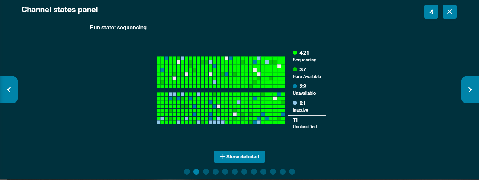
- Large amount of pores in the Inactive state. It has been advised from David Eccles (see this post here) that a large amount of inactive pores in random spots indicates a defective flow cell (example here). Issues with sample preparation and the introduction of air bubbles can cause pores to be inactive, however, this is more likely to occur in distinct regions of the flow cell. It is advised that you start a sequencing run without adding any flush buffer or sample to see how many pores are "available" at the start of your run, then load as necessary. You should see a sea of green pores at the start with no issues (example here).
- Sequencing RNA will always have a decent number of pores sequencing adapter. Per ONT here: "For RNA in particular, the expanded channels view may show a large proportion of pores sequencing Adapter. This happens because RNA strands are usually shorter than DNA, and the adapter takes up a larger proportion of the strand. Additionally, the RNA sequencing chemistry is optimised for sequencing RNA, whereas the adapter is DNA, and is processed slower. As long as the 'basic' pore activity plot view shows the majority of pores in "Sequencing", a high proportion of Adapter should not be a problem."
- According to Kanhav Khanna, an ONT tech, total RNA and mRNA perform the same for human but not for other species. In my discussions with him, some individuals have reported better results with mRNA (for instance, when studying RNA from yeast), but this hasn't been the case with human RNA. This appears to reflect my runs thus far.
- For the Flongle, aim to load 3-20 fmol of RNA; 10-15 fmol ideally. This can be calculated using the NEBio RNA mass calculator, or the formula on that page. Typically, the average RNA length (N50) is around 1,400 bases, so substitute that into the formula and 10 fmol to determine what amount you should load in ng.
- "Wildflower" Pattern and Flow Cell Quality. Some flow cells appear to have a "wildflower pattern" as it is known on the ONT community forums, since the flow cell has many pores in different states (Active Feedback, Inactive, Sequencing, Adapter, Zero, etc.). You may find a discussion about this on the forums here. As noted by a user, "The good flow cells seem to have a high number of pores at initial check (~1600) whereas flow cells just above the warranty tend to fall off quickly. I saw it with flongles too, those with >80 pores were great, those starting around ~50 died quickly. It seems to be a quality control thing." You should start "sequencing" on your flow cell always to truly check the flow cell's status prior to sample loading.
- Quick Pore Decay can be due to a Number of Factors. Some of these include: large amounts of fragmented RNA/DNA in the sample (you can check this by mapping the control RCS RNA in the Direct RNA Sequencing kit and looking for fragmentation), contaminants present in your sample (detergents, proteins, etc.), poor flow cell quality (flow cells that are old and have been sitting for more than a month, or have low pore availability even if above warranty; see "wildflower" comment above), overloading the flow cell, and/or damaging the pores upon sample loading.
| Pore Status | Description |
|---|---|
| Sequencing | Indicates that the pore is currently sequencing. This is the ideal state. Can be either "adapter" sequencing or "strand" sequencing. You can figure out which it is by clicking the "show detailed" box. |
| Pore Available | This means that the pore is available for sequencing, but no strand is currently being sequenced. A large portion of pores in this state usually indicates that you have loaded a small amount of library. |
| Adapter | The pore is sequencing the unligated sequencing adapter only. Reads will initially be classified as adapter until the DNA/RNA strand starts translocating through the pore and MinKNOW is able to reclassify the read. A large portion of adapters sequencing relative to actual sample RNA means that your library preparation was pore. |
| No Pore | No pore was detected in the channel. |
| Unavailable | The channel appears to show a pore that is currently unavailable for sequencing. |
| Unclassified | Pore status unknown. |
| Saturated | The channel has switched off due to current levels exceeding hardware limitations. |
| Out of range-high | Current is positive (between 10 and 9999 pA) and unavailable for sequencing. |
| Out of range-low | Current is negative (between -5 and -9999 pA) and unavailable for sequencing. |
| Zero | Pore currently unavailable for sequencing and the current level is between -5 and 10 pA. According to ONT specialist Kanhav Khanna, this is usually due to osmotic imbalance caused by an air bubble or some detergent in the sample. Look for "swaths" or patches of pores in the Zero state, which may indicate an air bubble in that location. |
| Multiple | Multiple pores detected. Unavailable for sequencing. |
| Active Feedback | The channel is reversing the current flow to eject the analyte (DNA/RNA). |
Additional Information
One last thing I wanted to include in this protocol is a list of useful information I have found regarding running mRNA samples through the nanopore. This includes references to the ONT documentation (which may require a login to access the original source) as well as publications. Reference back to it as necessary.
- Poly(A) Tail Required for Sequencing: According to ONT, a poly(A) tail is required for the preparation of the RNA sequencing library. Some RNA molecules, such as long-non-coding RNAs (lncRNAs), rRNAs, tRNAs, and some of your controls (i.e. G. Luciferase and C. Luciferase RNAs) will therefore not be read. It is important, then, to add a poly(A) tail to these molecules enzymatically in vitro prior to the generation of the RNA library using an E. coli poly(A) polymerase (NEB Cat No.: M0276L). Details about this procedure can be found in the ONT Documentation, which also shows a few graphs suggesting optimum incubation time (0.5-1.5 min) at 37ºC (ONT Docs: RNA Polyadenylation).
- Poly(A) Tail Length Bias: ONT has noted in their documentation that there may be a yield bias for mRNAs that have longer poly(A) tails in yeast, but it seems that this may not be the case for humans. Please consult the documentation for more (ONT Docs: Poly(A) Enrichment).
- RNA Contaminants: Various chemicals used in the extraction procedure, including Phenols, Ethanol, Isopropanol, EDTA, NaCl, etc. can affect your RNA. Details of these effects can be found in the ONT Documentation, but the bottom line is that you should avoid contamination during library preparation at all costs (ONT Docs: RNA Contaminants). Additionally, contaminants in your RNA sample may also block the pores in your flow cell, leading to a lot of pores being placed in recovery (blue). NOTE: RNA contaminants, in my experience, and RNA quality greatly affect pore decay. Please see the "RNA Sample Quality and Throughput" point below for more.
- RNA Read Direction 3’->5’: In the RNA sequencing protocol, ONT notes the following: “Please note that, unlike DNA, RNA is translocated through the nanopore in the 3’-5’ direction. However, the basecalling algorithms automatically flip the data, and the reads are displayed 5’-3’.” Useful to keep in mind.
- RNA Stability in Storage: ONT describes in their documentation the stability of RNA over time. If stored properly, RNA should remain relatively stable in the proper buffers at -20ºC for 200+ days (ONT Docs: RNA Stability).
- RNA Stability during Sequencing: RNA will degrade during the sample run over time. Workman et al. found that RNA sequences degrade over the course of a 36 hour run, but this effect was minimal (~5%) in mitochondrial control RNAs over this period, suggesting that a run over the course of 24 hours should exhibit negligible degradation (Workman et al. 2019).
- RNA Sample Quality and Throughput: It is advised that the RNA samples be evaluated for quality via an RNA Integrity Number (RIN) (7+/10) prior to sequencing using an Agilent 2100 Bioanalyzer. This equipment can be pretty pricey, though. Your final RNA library to be sequenced via nanopore should be around 20 ng/uL for a good output. I have found that contaminants and RNA quality greatly affect throughput and pore decay. To avoid this, you should do two things: 1) dilute the input mRNA (before library prep) to around 300 ng / 9 µL and load 9 µL directly. 2) Check the RNA quality via nanodrop and make sure the interpreted results indicate a good RNA sample.
- M6ANet Requires a Minimum of 20 Reads: According to the author here, m6ANet will not generate any inferences for mapped transcripts with fewer than 20 reads. This is a limitation of the software.
- M6ANet Mod Probability: According to the author here, the m6ANet mod probability represents the probability that the modification at that site would be picked up using m6ACE.
- M6ANet Mod Ratio: Again, according to the author here, the m6ANet mod ratio represents the ratio of m6A modifications found to be modified 'using' the m6ANet mod probability. Therefore, mod ratio and mod probability should be positively correlated.
- RNA Read Errors by Base: RNA nanopore reads have higher error rates than for DNA nanopore reads. Additionally, not all basecalling errors are the same. For instance, the nanopore system has a higher error rate confusing C-to-U (3.62%) and U-to-C (2.23%) than G-for-C (0.38%) and C-for-G (0.47%) with Albacore (Workman et al. 2019).
- RNA Read Truncation: In the Workman et al. study, it was also found that there were a number of truncated reads in their mitochondrial poly(A) transcripts, which were used as a control (since they are abundant, vary in length from 349-2,379 nucleotides, and are a single exon). They hypothesize that some possible non-biological causes of this include: 1) the last handful of nucleotides are not read when the pore translocation enzyme detaches the strand near the end, which causes the strand to rapidly move through the pore, 2) ionic current signal artifacts due to enzyme stalls during RNA translocation, or 3) RNA strand breaks (Workman et al. 2019).
- RNA m6A Controls: The Workman et al. study also used an m6A synthetic oligomer (FLuc) as a control for m6A detection. Very useful for you. It is described in the Oligomer Ligation section of the Methods in their paper (Workman et al. 2019).
- Wash Kits do not contain DNase: It appears that the flow cell wash kits do not contain DNase, per some discussions that took place in the comments here. Therefore, it is not likely that your washes will recover flow cell pores following direct RNA sequencing. Perhaps try adding in some RNase?
Appendix
- Alignment: A process by which a given DNA or RNA sequence is matched with a reference genome / transcriptome, and therefore given a gene name.
- Bam: A type of DNA or RNA sequencing file containing your reads after they have been mapped to the genome. It is a binary version of the earlier .SAM file, which is where it gets its name.
- Bam.bai: An index file with the same prefix name as a .bam file. This file acts like an external table of contents, which allows algorithms and software to be able to jump to specfic sections of the .bam file without having to read through all the sequences.
- Basecalling: A term used to refer to the process of obtaining direct measurements of ionic current as DNA/RNA is fed through a nanopore, and then using that information to obtain DNA/RNA nucleotide “reads”. Basecalling is achieved by running the raw Fast5 files through the Guppy software.
- Conda: A collection of tools and runtime environment for installing software on a home machine.
- CUDA: Stands for “Compute Unified Device Architecture”, which allows GPU resources to be used for general processing. Developed by and for NVIDIA GPUs.
- Docker: A Linux container whereby you can run Linux code and commands in a virtual environment. I originally used this with an earlier version of this protocol, but it may not be required anymore. Alternative to singularity.
- Fast5: A type of raw file obtained from sequencing DNA or RNA molecules. This can be converted into a Fastq file using the Guppy software provided by Oxford Nanopore.
- Fastq: A type of raw file obtained from sequencing DNA or RNA molecules and houses the sequenced genetic material. Fastq files are often a processed step up from Fast5 files, since they contain some metadata about the sequenced material.
- Flow cell: A term used for the sheet that contains the nanopores that sequence DNA/RNA data, along with their electrodes and sensor chip.
- Guppy: Guppy is a basecalling algorithm provided by Oxford Nanopore Technologies, which reads the fast5 or fastq files obtained from the Oxford Nanopore (such as “MinION”), and generates the DNA/RNA bases.
- MinION / GridION: Two different hardware enclosures that house ONT flow cells while sequencing is occurring and relays that information to a computer.
- Nanopore: Microscopic protein pores embedded in an electrically-resistant polymer membrane and used to process DNA/mRNA strands.
- Nuclease-free Water: Water that has been purified to not be contaminated by non-sample nucleases. This is important for gene sequencing and PCR protocols, to ensure that the material you are working with is only from your sample.
- ONT: A reference to “Oxford Nanopore Technologies”, the manufacturer of the Nanopore we use in the lab. You will see this in a lot of folders that house files from the company, such as “ont-guppy”, which is used to sequence raw nanopore data.
- Python: A type of programming language.
- R: Programming language commonly used by scientists to analyze data.
- Reads: Term used to refer to sequenced genetic material (DNA or RNA).
- Root Folder: The parent folder location that houses most of your files. For the purposes of these guides, we are considering the root folder at
/home/username/(Linux) or/Users/username(Mac). Denoted by “root” or~. - .SAM: A type of file format that holds processed sequencing data. Stands for “Sequence Alignment Map format”.
- Shell Script: A series of code that can be executed at once via the shell (i.e. in Terminal).
- Singularity: A Linux container whereby you can run Linux code and commands in a virtual environment. Alternative to docker.
- Terminal: An application on both Linux and Mac machines that gives you access to the shell whereby you can execute commands.
- XCode: Integrative Development Environment and collection of programming tools provided by Apple, Inc. for developing software.